One of the images in this post is a little graphic. Do not click on the last image if you wish to avoid seeing it.
Introduction
Have you heard of AWS Lookout for Vision ? It is a really cool service that AWS unveiled in December 2020 during their Re:Invent conference. It automatically trains a machine learning model for detecting anomalies and defects in a production line. All you have to do is provide it with a couple hundred images from the parts on your production line that you classify as either normal or anomalous and Lookout for Vision does everything else for you, from training the model all the way to hosting it.
Sounds pretty amazing, doesn't it? This can be used to easily automate a lot of quality control at low cost. However, as is often the case in deep learning, the devil is in the details and knowing how reliable your model's performance really is can be more involved than simply looking at the test accuracy. Let's take a look at what can go wrong.
Warm-up Example
Before tackling any real dataset I want to illustrate the difficulty of out-of-distribution detection on a very simple example. For that, we will look at MNIST - a hand-written digit recognition task and (in)famously baby's first deep learning dataset. We will pick out just the digits "8" and "1" and label them as follows: we call all "8"s "normal" and all "1"s anomalous.


Now we feed this training data into Lookout for Vision and let it do its thing. The final classifier ends up having perfect accuracy on the test set. It doesn't make even a single mistake. However, in practice there could be all sorts of anomalies that we never had in our training or test set. Let's say that a camera breaks completely and we end up sending only uniform noise to the model, as shown below.


It turns out that both of these images get classified as "normal" by the Lookout for Vision model, even though they clearly look nothing like the digit "8". In the histogram below I show the confidence in the normal class (negative confidence means a correct classification as "anomalous"). As you can see almost all noise samples end up being classified as normal.

What went wrong here? Well, the model learned from the training data that normal samples always have more white pixels than anomalous ones. This made the model overfit on this spurious feature so that the uniform noise images got misclassified, despite being extremely obvious outliers to humans. In this toy example it is very easy to understand this failure mode but on more complicated datasets, the spurious features could be much more complicated.
Now on actual Data
Since MNIST is really not the most interesting dataset, let's try our hands on actual images of actual parts from an actual production line. Helpfully, AWS provides a Hello World dataset for us where we ask the model to classifiy circuit boards into normal and anomalous. Here are examples of normal and anomalous parts:
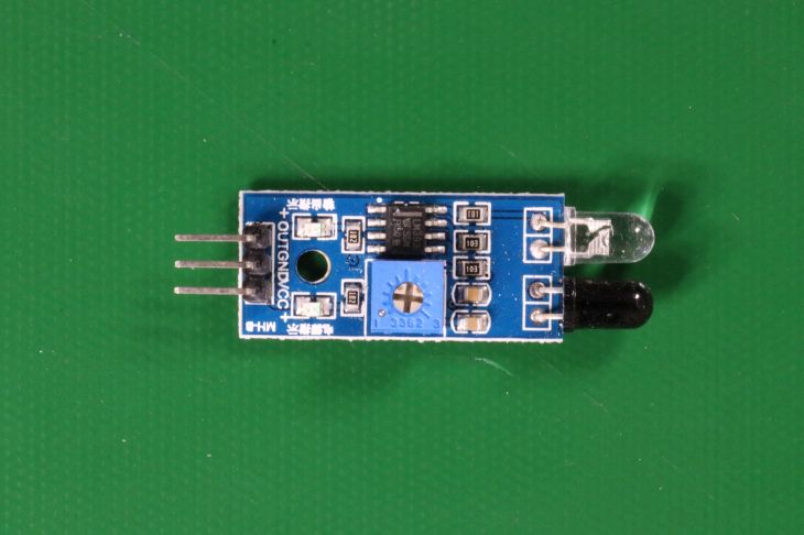

The differences here are quite subtle. The anomalous part on the right happens to have some soldering tin on the potentiometer in the middle of the part. Lookout for Vision is able to pick up on these small anomalies and two out of the three models I trained ended up having perfect accuracy on the test set. Impressive feat, considering that the images have a resolution of a whopping 4000x2667 pixels and the training set isn't very big.
But now let's check for interesting failure cases. First, let's try to throw images of objects at the model that it has never seen before and see how it does. Out of 5000 images (all taken from the imagenet test set ) only three were incorrectly predicted to be "normal". Below, you can see an example. Clearly, that's not a circuit.

But we can go even further. We can also take an image that is correctly labeled as anomalous and then modify it just a little bit until the model believes that it's seeing a normal circuit board. This is known as an Adversarial Attack and since we do not have direct access to the model parameters but only to the model outputs, we say that it is running in a black-box setting. I ran the popular black-box attack Square Attack and after only 161 updates to the image I could convince the model that this pile of fruit is actual an electronics component that's ready to be sold. On the left you see the original, on the right the modified image. The difference is almost invisible to a human but huge for the AI.


This is all well and good, but you might say that none of these images are at all related to the environment where we are deploying the model. So who cares? Well, let's try to craft some examples that might actually occur in practice. First, we remove the electronics component from a test image so that we can use the background as a canvas. This image correctly gets identified as anomalous. If I run the Square Attack again I can actually start fooling the model after only 4 changes to the image. The original and modified images are shown below.

Since this worked so well, we can try to put some objects on the canvas and see if that fools the model. Let's try an object that we really, really wouldn't want to sell in place of a circuit board. If you place our adversarial object at just the right angle at just the right location and just the right scale then you can, in fact, convince the model that the image below is an image of a perfectly acceptable circuit board. You really wouldn't want that shipped to a customer.

Since the model works at very high resolution and in a very low data regime, one would expect some amount of adversarial vulnerability, but in all fairness, finding these vulnerabilities ended up being much harder than I would have anticipated. Not just any adversarial attack algorithm works and not all samples could easily be manipulated to yield failure cases.
Conclusion
So what do we learn from this? Well, we learned that it can be really difficult to fully evaluate the weaknesses of a machine learning system. 100% accuracy doesn't always tell the full story. In this example, we likely don't have to fear that some nefarious actor tries to manipulate our system in a way that it makes undesirable decisions but there can certainly be applications where we really need to be sure that our machine learning system is safe and reliable.